Modules of methods of calculation
Tight-Binding method
Semiempirical Tight Binding method was realized.
- class kvazar.core.tb.TB(struct, parm)[source]
Class that realizes Tight-Binding method.
Constructor of class TB.
Args:
struct (Structure): nanostructure.
lib (module): dynamic library, it realize filling Hamiltonian matrix, calculating repulsive energie, forces acting on atoms.
parms (dict): parameters of method.
Kwargs:
functions (list): list of functions that will be loaded from lib library.- compute()[source]
Calculating full energy of nanostructure.
Returns:
energy_total(float): full energy of nanostructure
- compute_ebond()[source]
Calculating bond energy using formula
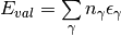
where
 is a value on diagonal of diagonalised hamiltonian
Returns:
energy_bond(float): bond energy of atoms
- compute_erep()[source]
Repulsive energy between two atoms

Total repulsive energy
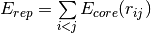
- Returns:
- energy_rep(float): repulsive energy
- ensure_forces()[source]
Function changes method for calculating forces, acting on atoms of structure, to ensure, that hamiltonian matrix is not zero before calculation start and eigenvectors can be calculated.
- load_force_function(lib)[source]
Loading of function that calculate forces and creating wrap-methods from dynamic library.
Args:
functions (list): list of functions, that will be loaded from lib
lib (module): dynamic library
- load_tb_functions(functions, lib)[source]
Loading of functions from dynamic library and creating wrap-methods.
Args:
functions (list): list of functions, that will be loaded from lib
lib (module): dynamic library
- preprocessing(struct)[source]
Preprocessing for TB method, that:
- Checks existing of parameters for different atom types, involved in structure.
- Creates Hamiltonian matrix.
- Calculates number of orbitals of each type and shift indices for orbitals in hamiltonian.
- Calculates number of occupied energy levels
- Args:
- struct (Structure): nanostructure
Molecular mechanics
Molecular mechanics method was realized.
- class kvazar.core.mm.MM(struct, lib, ff_functions, ff_params)[source]
Wrap class for computational modules of molecular mechanical method.
Constructor of class:
Args:
struct(structure): nanostructure
lib(module): dynamic library
ff_functions(list): list of names of force field functions
ff_params(list): list of names of parameters of force field functions
- compute_ij(i, j)[source]
Returns summ of energies, calculated by functions from list ‘functions_ij’
- loadMMFunctions(ff_functions, lib)[source]
Args:
ff_functions(list): list of names of atom types
lib(module): dynamic library for molecular mechanics computation
- preprocessing(struct)[source]
It checks matching of atom types and atom names of structure with the same parameters of force field. If there are no atom types in structure function rebuilds it from atom names. If there are no atom names, it prints, that it’s not possible to check out correctness of atom types.
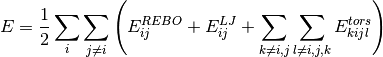
Reactive empirical bond order potential
Method REBO was realised according to article: Donald W. Brenner, Olga A. Shenderova, Judith A. Harrison, Steven J. Stuart, Boris Ni, and Susan B. Sinnott, “A second-generation reactive empirical bond order (REBO) potential energy expression for hydrocarbons” // J. Phys.: Condens. Matter 14(2002), P. 783–802. Description for method was taken from this article.
Chemical binding energy
can be written as a sum over nearest neighbours in the form:
(1)
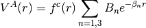
The equation (1) is used for the total potential energy. Following the earlier hydrocarbon bonding expression, the empirical bond order function used here is written as a sum of terms:
(2)
Values for the function
and
depend on the local coordination and bond angles for atoms
and
respectively. The function
is further written as a sum of two terms:
(3)
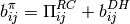
The first generation hydrocarbon expression used Morse-type terms for the pair interactions in equation (1). It was determined that this form is too restrictive to simultaneously fit equilibrium distances, energies, and force constants for carbon-carbon bonds. This form has the further disadvantage that both terms go to finite values as the distance between atoms decreases, limiting the possibility of modeling process involving energetic atomic collisions. In the second-generation potential next forms are used for attractive ad repulsive potentials:
(4)
and
(5)
Analytic forms for each term in equation (2) are fitted to both the discrete values of the bond orders above, and to other properties of solid-state and molecular carbon as described below. The first term in equation (2):
(6)
where
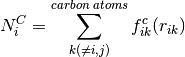
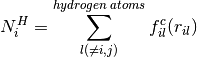
is a function to ensure that interations include only nearest neighbours. P represents a bicubic spline and quantities
and
represent the number of carbon and hydrogen atoms, respectively, that are neighbours of atom
(7)
and
(8)
The term
is taken as tricubic spline
:
(9)
is given by next expression:
(10)
where
(11)
and
(12)
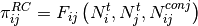
The term
in equation (3) :
(13)
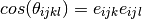
where
(14)
The function
is a tricubic spline,
and
are unit vectors in the direction of the cross products
and
, respecrively, where R are vectors connecting subscripted atoms.
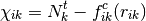
The value of
(15)
![E_b = \sum_{i}\sum_{j(>i)}[V^R(r_{ij}) - b_{ij}V^A(r_{ij})]](_images/math/3a425b52c60b7fd8b6e939fe630e9ad91a01e182.png)
![\overline{b}_{ij} = \frac{1}{2}[b_{ij}^{\sigma-\pi} + b_{ji}^{\sigma-\pi}] + b_{ij}^\pi](_images/math/7fe251955351055ba2dd8993dedc724c6653ff3b.png)

![b_{ij}^{\sigma-\pi} = \left[ 1 + \sum_{k(\ne i,j)}f^{c}_{ik}(r_{ik})G(cos(\theta_{ijk}))e^{\lambda_{ijk}} + P_{ij}(N^{C}_i , N^{H}_i)\right]^{-\frac{1}{2}}](_images/math/baa1a2ab441f36735995e6475604656e41fe3c99.png)
![N_{ij}^{conj} = 1 + \left[\sum_{k(\ne i,j)}^{carbon}f_{ik}^c (r_{ik})F(X_{ik}) \right] ^ 2 + \left[\sum_{l(\ne i,j)}^{carbon}f_{il}^c (r_{il})F(X_{il}) \right] ^ 2](_images/math/512dc2d15fa5e3a787d9d48eeb7ef2a1473244c3.png)
![$F(\chi_{ik}) = \begin{cases}
1 & \chi_{ik} < 2 \\
[1+cos(2\pi(\chi_{ik}-2))]/2 & 2 < \chi_{ik} < 3 \\
0 & \chi_{ik} > 3
\end{cases}$](_images/math/dc9c2848cfe6481f4e2902ad37b06c301803055d.png)
![b_{ij}^{DH} = T_{ij}(N_{i}^t ,N_{j}^t ,N_{ij}^{conj})\left[\sum_{k(\ne i,j)}\sum_{l(\ne i,j)}(1 - cos^{2}(\theta_{ijkl}))f_{ik}^{c}(r_{ik})f_{jl}^{c}(r_{il})\right]](_images/math/a01d497bf2168093240b2d42bdbfb5791dcb6243.png)
![$f_{ij}^{c}(r) = \begin{cases}
1 & r < D_{ij}^{min} \\
\left[ 1 + cos(\pi((r - D_{ij}^{min})/(D_{ij}^{max} - D_{ij}^{min}))\right]/2 & D_{ij}^{min} < r < D_{ij}^{max} \\
0 & r > D_{ij}^{max}
\end{cases}$](_images/math/d68ef60b564d485f192c44359ca1a2fbf34823d5.png)
Adaptive intermolecular reactive empirical bond order potential
AIREBO method was realized according to article: Steven J. Stuart, Alan B. Tutein and Judith A. Harrison. “A reactive potential for hydrocarbons with intermolecular interactions” // Journ. of Chem. Phys., V 112,14 (2000), p. 6472-6486.
AIREBO potential can be represented by a sum over pairwise interactions, including covalent bonding REBO interactions, LJ terms, and torsion interactions:
(16)
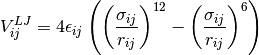
Van-der-Vaals interaction is described through the using of the Lennard-Jones potential:
(17)
is the traditional LJ term:
(18)
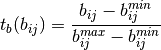
It was modified by several sets of switching functions. S(t) can be represented in the next form:
(19)
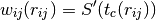
Magnitude of LJ interactions depends on bonding environment. Gradual exclusion of Lennard-Jones interactions with changings of
is controlled by scalling function
:
(20)
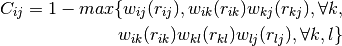
If atoms
(21)
where:
The torsional part of equation (16) for the dihedral angle determined by atoms i, j, k, l has the next form:
(22)
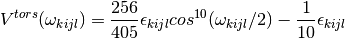
where
is the torsional potential:
(23)
- class kvazar.core.airebo.AIREBO(struct, ff_params, comm=None)[source]
This class is the successor of class MM
Constructor of class AIREBO:
Args:
struct(structure): nanostructure
ff_params(list): list of names of potentials functions
- init_cutoff(r_in, r_out, cutoff_neighbours)[source]
Args:
r_in(float): internal cutoff radius
r_out(float): external cutoff radius
cutoff_neighbours(list): list of neighbours get into the field with r_out radius
![E_{ij}^{LJ} = S(t_r (r_{ij}))S(t_b (b_{ij}^* ))C_{ij}V_{ij}^{LJ}(r_{ij}) + [1 - S(t_r(r_{ij}))]C_{ij}V_{ij}^{LJ}(r_{ij})](_images/math/24ce40c7db56764cdda23c15a2918773b861ac1c.png)
![S(t) = \Theta(-t)+\Theta(t)\Theta(1-t)[1 - t^2(3-2t)]](_images/math/ba5019f6772dce35efdcb47779aa5022da277b44.png)
![S^\prime(t_c(r_{ij})) = \Theta(-t)+\Theta(t)\Theta(1-t)\frac{1}{2}[1+cos(\pi t)]](_images/math/6fcadd7fb090ae3db8ee608de29441e63079a1bf.png)

Coarse-grained modeling
MARTINI force field for coarse-grained modeling was realized.
- class kvazar.core.martini.MARTINI(struct, ff_params)[source]
This class is the successor of class MM
Constructor of class MARTINI:
Args:
struct(structure): nanostructure
ff_params(list): list of names of force field parameters(functions)
- init_cutoff(r_in, r_out, cutoff_neighbours)[source]
Args:
r_in(float): internal cutoff radius
r_out(float): external cutoff radius
cutoff_neighbours(list): list of neighbours get into the field with r_out radius